Square root of a matrix
In mathematics, the square root of a matrix extends the notion of square root from numbers to matrices. A matrix B is said to be a square root of A if the matrix product B · B is equal to A.[1]
Contents |
Properties
In general, a matrix can have many square roots. For example, the matrix  has square roots
  and
and  , as well as their additive inverses. Another example is the 2×2 identity matrix
  which has an infinitude of symmetric rational square roots given by


 and
and  where (r, s, t) is any Pythagorean triple — that is, any set of positive integers such that
  [2]
[2]
However, a positive-definite matrix has precisely one positive-definite square root, which can be called its principal square root.
While the square root of an integer is either again an integer or an irrational number, in contrast an integer matrix can have a square root whose entries are rational, yet not integral. For example, the matrix  has a square root
  , as well as a square root that is an integer matrix:
  . The other two square roots are the additive inverses of these (In general, a 2×2 matrix with two distinct eigenvalues has four square roots). The 2×2 identity matrix discussed above provides another example.
Just as with the real numbers, a real matrix may fail to have a real square root, but have a square root with complex-valued entries.
Computation methods
Explicit formulas
For a 2 × 2 matrix, there are explicit formulas that give up to four square roots, if the matrix has any roots.
If D is a diagonal n × n matrix, one can obtain a square root by taking a diagonal matrix R, where each element along the diagonal is a square root of the corresponding element of D. If the diagonal elements of D are real and non-negative, and the square roots are taken with non-negative sign, the matrix R will be the principal root of D.
By diagonalization
An n × n matrix A is diagonalizable if there is a matrix V and a diagonal matrix D such that  . This happens if and only if A has n eigenvectors which constitute a basis for Cn. In this case, V can be chosen to be the matrix with the n eigenvectors as columns, and a square root of
  is
is
where S is any square root of D. Indeed,

For example, the matrix  can be diagonalized as
  , where
 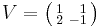 and
and 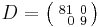 .
.
 has principal square root
 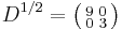 , giving the square root
 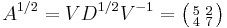 .
.
By Jordan decomposition
For non-diagonalizable matrices one can calculate the Jordan normal form followed by a series expansion, similar to the approach described in logarithm of a matrix.
By Denman–Beavers iteration
Another way to find the square root of an n × n matrix A is the Denman–Beavers square root iteration. Let Y0 = A and Z0 = I, where I is the n × n identity matrix. The iteration is defined by
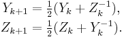
Convergence is not guaranteed, even for matrices that do have square roots, but if the process converges, the matrix  converges quadratically to a square root A1/2, while
  converges to its inverse, A−1/2. (Denman & Beavers 1976; Cheng et al. 2001).
By the Babylonian method
Yet another iterative method is obtained by taking the well-known formula of the Babylonian method for computing the square root of a real number, and applying it to matrices. Let X0 = I, where I is the identity matrix. The iteration is defined by
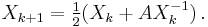
Again, convergence is not guaranteed, but if the process converges, the matrix  converges quadratically to a square root A1/2. Compared to Denman–Beavers iteration, an advantage of the Babylonian method is that only one matrix inverse need be computed per iteration step. However, unlike Denman–Beavers iteration, this method is numerically unstable and more likely to fail to converge.[1]
Square roots of positive operators
In linear algebra and operator theory, given a bounded positive semidefinite operator (a non-negative operator) T on a complex Hilbert space, B is a square root of T if T = B* B, where B* denotes the Hermitian adjoint of B. According to the spectral theorem, the continuous functional calculus can be applied to obtain an operator T½ such that T½ is itself positive and (T½)2 = T. The operator T½ is the unique non-negative square root of T.
A bounded non-negative operator on a complex Hilbert space is self adjoint by definition. So T = (T½)* T½. Conversely, it is trivially true that every operator of the form B* B is non-negative. Therefore, an operator T is non-negative if and only if T = B* B for some B (equivalently, T = CC* for some C).
The Cholesky factorization provides another particular example of square root, which should not be confused with the unique non-negative square root.
Unitary freedom of square roots
If T is a non-negative operator on a finite dimensional Hilbert space, then all square roots of T are related by unitary transformations. More precisely, if T = AA* = BB*, then there exists a unitary U s.t. A = BU.
Indeed, take B = T½ to be the unique non-negative square root of T. If T is strictly positive, then B is invertible, and so U = B−1A is unitary:
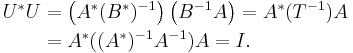
If T is non-negative without being strictly positive, then the inverse of B cannot be defined, but the Moore–Penrose pseudoinverse B+ can be. In that case, the operator B+A is a partial isometry, that is, a unitary operator from the range of T to itself. This can then be extended to a unitary operator U on the whole space by setting it equal to the identity on the kernel of T. More generally, this is true on an infinite-dimensional Hilbert space if, in addition, T has closed range. In general, if A, B are closed and densely defined operators on a Hilbert space H, and A* A = B* B, then A = UB where U is a partial isometry.
Some applications
Square roots, and the unitary freedom of square roots have applications throughout functional analysis and linear algebra.
Polar decomposition
If A is an invertible operator on a finite-dimensional Hilbert space, then there is a unique unitary operator U and positive operator P such that

this is the polar decomposition of A. The positive operator P is the unique positive square root of the positive operator A∗A, and U is defined by U = AP−1.
If A is not invertible, then it still has a polar composition in which P is defined in the same way (and is unique). The unitary operator U is not unique. Rather it is possible to determine a "natural" unitary operator as follows: AP+ is a unitary operator from the range of A to itself, which can be extended by the identity on the kernel of A∗. The resulting unitary operator U then yields the polar decomposition of A.
Kraus operators
By Choi's result, a linear map
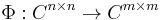
is completely positive if and only if it is of the form
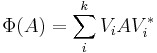
where k ≤ nm. Let {Ep q} ⊂ Cn × n be the n2 elementary matrix units. The positive matrix
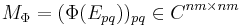
is called the Choi matrix of Φ. The Kraus operators correspond to the, not necessarily square, square roots of MΦ: For any square root B of MΦ, one can obtain a family of Kraus operators Vi by undoing the Vec operation to each column bi of B. Thus all sets of Kraus operators are related by partial isometries.
Mixed ensembles
In quantum physics, a density matrix for an n-level quantum system is an n × n complex matrix ρ that is positive semidefinite with trace 1. If ρ can be expressed as
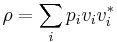
where ∑ pi = 1, the set

is said to be an ensemble that describes the mixed state ρ. Notice {vi} is not required to be orthogonal. Different ensembles describing the state ρ are related by unitary operators, via the square roots of ρ. For instance, suppose
The trace 1 condition means
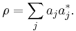
Let

and vi be the normalized ai. We see that
gives the mixed state ρ.
See also
Notes
- ^ a b Higham, Nicholas J. (April 1986). "Newton's Method for the Matrix Square Root". Mathematics of Computation 46 (174): 537–549. doi:10.2307/2007992. http://www.ams.org/journals/mcom/1986-46-174/S0025-5718-1986-0829624-5/S0025-5718-1986-0829624-5.pdf.
- ^ Mitchell, Douglas W. "Using Pythagorean triples to generate square roots of I2". The Mathematical Gazette 87, November 2003, 499-500.
Bibliography
- Cheng, Sheung Hun; Higham, Nicholas J.; Kenney, Charles S.; Laub, Alan J. (2001), "Approximating the Logarithm of a Matrix to Specified Accuracy", SIAM Journal on Matrix Analysis and Applications 22 (4): 1112–1125, doi:10.1137/S0895479899364015, http://www.eeweb.ee.ucla.edu/publications/journalAlanLaubajlaub_simax22(4)_2001.pdf
- Denman, Eugene D.; Beavers, Alex N. (1976), "The matrix sign function and computations in systems", Applied Mathematics and Computation 2 (1): 63–94, doi:10.1016/0096-3003(76)90020-5
- Burleson, Donald R., Computing the square root of a Markov matrix: eigenvalues and the Taylor series, http://www.blackmesapress.com/TaylorSeries.htm